Branching Reader
This notebook demonstrates the capability of the serpentTools package to read branching coefficient files. The format of these files is structured to iterate over:
Branch states, e.g. burnup, material properties
Homogenized universes
Group constant data
The output files are described in more detail on the SERPENT Wiki
Basic Operation
Note
The preferred way to read your own output files is with the
serpentTools.read() function. The serpentTools.readDataFile() function is used here
to make it easier to reproduce the examples
Note
Without modifying the settings, the
BranchingReader assumes that all
group constant data is presented without the associated uncertainties.
See User Control for examples on the various ways to
control operation
>>> import serpentTools
>>> branchFile = 'demo.coe'
>>> r0 = serpentTools.readDataFile(branchFile)
The branches are stored in custom dictionary-like BranchContainer
objects in the branches dictionary
>>> r0.branches.keys()
dict_keys([
    ('nom', 'nom'),
    ('B750', 'nom'),
    ('B1000', 'nom'),
    ('nom', 'FT1200'),
    ('B750', 'FT1200'),
    ('B1000', 'FT1200'),
    ('nom', 'FT600'),
    ('B750', 'FT600'),
    ('B1000', 'FT600')
])
Here, the keys are tuples of strings indicating what
perturbations/branch states were applied for each SERPENT solution.
Examining a particular case
>>> b0 = r0.branches['B1000', 'FT600']
>>> print(b0)
<BranchContainer for B1000, FT600 from demo.coe>
SERPENT allows the user to define variables for each branch through
var V1_name V1_value cards. These are stored in the
stateData attribute
>>> b0.stateData
{'BOR': '1000',
 'DATE': '17/12/19',
 'TFU': '600',
 'TIME': '09:48:54',
 'VERSION': '2.1.29'}
The keys 'DATE', 'TIME', and 'VERSION' are included by
default in the output, while the 'BOR' and 'TFU' have been
defined for this branch.
Group Constant Data
Note
Group constants are converted from SERPENT_STYLE to
mixedCase to fit the overall style of the project.
The BranchContainer stores group constant data in HomogUniv objects as a dictionary.
>>> for key in b0:
...     print(key)
UnivTuple(universe='0', burnup=0.0, step=0, days=None)
UnivTuple(universe='10', burnup=0.0, step=0, days=None)
UnivTuple(universe='20', burnup=0.0, step=0, days=None)
UnivTuple(universe='30', burnup=0.0, step=0, days=None)
UnivTuple(universe='40', burnup=0.0, step=0, days=None)
UnivTuple(universe='0', burnup=1.0, step=1, days=None)
UnivTuple(universe='10', burnup=1.0, step=1, days=None)
UnivTuple(universe='20', burnup=1.0, step=1, days=None)
UnivTuple(universe='30', burnup=1.0, step=1, days=None)
UnivTuple(universe='40', burnup=1.0, step=1, days=None)
UnivTuple(universe='0', burnup=10.0, step=2, days=None)
UnivTuple(universe='10', burnup=10.0, step=2, days=None)
UnivTuple(universe='20', burnup=10.0, step=2, days=None)
UnivTuple(universe='30', burnup=10.0, step=2, days=None)
UnivTuple(universe='40', burnup=10.0, step=2, days=None)
The keys here are UnivTuple instances
indicating the universe ID, and point in the burnup schedule.
These universes can be obtained by indexing this dictionary, or by using
the getUniv() method
>>> univ0 = b0["0", 1, 1, None]
>>> print(univ0)
<HomogUniv 0: burnup: 1.000 MWd/kgu, step: 1>
>>> univ0.name, univ0.bu, univ0.step, univ0.day
('0', 1.0, 1, None)
>>> univ1 = b0.getUniv('0', burnup=1)
>>> univ2 = b0.getUniv('0', index=1)
>>> univ0 is univ1 is univ2
True
Group constant data is spread out across the following sub-dictionaries:
infExp: Expected values for infinite medium group constantsinfUnc: Relative uncertainties for infinite medium group constantsb1Exp: Expected values for leakage-corrected group constantsb1Unc: Relative uncertainties for leakage-corrected group constantsgc: Group constant data that does not match theINFnorB1scheme
For this problem, only expected values for infinite and critical
spectrum (b1) group constants are returned, so only the infExp and
b1Exp dictionaries contain data
>>> univ0.infExp
{'infDiffcoef': array([ 1.83961 ,  0.682022]),
 'infFiss': array([ 0.00271604,  0.059773  ]),
 'infS0': array([ 0.298689  ,  0.00197521,  0.00284247,  0.470054  ]),
 'infS1': array([ 0.0847372 ,  0.00047366,  0.00062865,  0.106232  ]),
 'infTot': array([ 0.310842,  0.618286])}
>>> univ0.infUnc
{}
>>> univ0.b1Exp
{'b1Diffcoef': array([ 1.79892 ,  0.765665]),
 'b1Fiss': array([ 0.00278366,  0.0597712 ]),
 'b1S0': array([ 0.301766  ,  0.0021261 ,  0.00283866,  0.470114  ]),
 'b1S1': array([ 0.0856397 ,  0.00051071,  0.00062781,  0.106232  ]),
 'b1Tot': array([ 0.314521,  0.618361])}
>>> univ0.gc
{}
>>> univ0.gcUnc
{}
Group constants and their associated uncertainties can be obtained using
the get() method.
>>> univ0.get('infFiss')
array([ 0.00271604,  0.059773  ])

>>> try:
...     univ0.get('infS0', uncertainty=True)
>>> except KeyError as ke:  # no uncertainties here
...     print(str(ke))
'Variable infS0 absent from uncertainty dictionary'
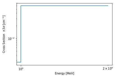
Plotting Universe Data
HomogUniv objects are capable of plotting homogenized data using the
plot() method. This method is tuned to plot group constants, such as
cross sections, for a known group structure. This is reflected in the
default axis scaling, but can be adjusted on a per case basis. If the
group structure is not known, then the data is plotted simply against
bin-index.
>>> univ0.plot('infFiss');
>>> univ0.plot(['infFiss', 'b1Tot'], loglog=False);
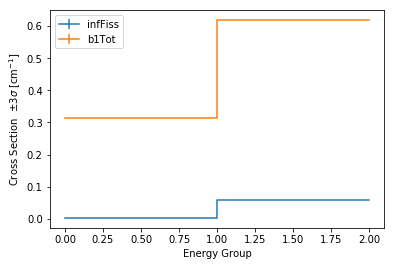
The ResultsReader example has a more thorough example of this plot()
method, including formatting the line labels - Plotting universes.
Iteration
The branching reader has a
iterBranches()
method that works to yield branch names and their associated
BranchContainer objects. This can
be used to efficiently iterate over all the branches presented in the file.
>>> for names, branch in r0.iterBranches():
...     print(names, branch)
('nom', 'FT1200') <BranchContainer for nom, FT1200 from demo.coe>
('B1000', 'FT1200') <BranchContainer for B1000, FT1200 from demo.coe>
('B750', 'FT600') <BranchContainer for B750, FT600 from demo.coe>
('nom', 'nom') <BranchContainer for nom, nom from demo.coe>
('B750', 'FT1200') <BranchContainer for B750, FT1200 from demo.coe>
('B1000', 'FT600') <BranchContainer for B1000, FT600 from demo.coe>
('nom', 'FT600') <BranchContainer for nom, FT600 from demo.coe>
('B1000', 'nom') <BranchContainer for B1000, nom from demo.coe>
('B750', 'nom') <BranchContainer for B750, nom from demo.coe>
User Control
The SERPENT
set coefpara
card already restricts the data present in the coefficient file to user
control, and the BranchingReader includes similar control.
In our example above, the BOR and TFU variables represented
boron concentration and fuel temperature, and can easily be cast into
numeric values using the branching.intVariables and
branching.floatVariables settings. From the previous example, we see
that the default action is to store all state data variables as strings.
>>> assert isinstance(b0.stateData['BOR'], str)
As demonstrated in the Group Constant Variables example, use of
xs.variableExtras and xs.variableGroups controls what data is
stored on the HomogUniv
objects. By default, all variables present in the coefficient file are stored.
>>> from serpentTools.settings import rc
>>> rc['branching.floatVariables'] = ['BOR']
>>> rc['branching.intVariables'] = ['TFU']
>>> rc['xs.getB1XS'] = False
>>> rc['xs.variableExtras'] = ['INF_TOT', 'INF_SCATT0']
>>> r1 = serpentTools.readDataFile(branchFile)
>>> b1 = r1.branches['B1000', 'FT600']
>>> b1.stateData
{'BOR': 1000.0,
 'DATE': '17/12/19',
 'TFU': 600,
 'TIME': '09:48:54',
 'VERSION': '2.1.29'}
>>> assert isinstance(b1.stateData['BOR'], float)
>>> assert isinstance(b1.stateData['TFU'], int)
Inspecting the data stored on the homogenized universes reveals only the variables explicitly requested are present
>>> univ4 = b1.getUniv("0", 0)
>>> univ4.infExp
{'infTot': array([ 0.313338,  0.54515 ])}
>>> univ4.b1Exp
{}
Conclusion
The BranchingReader is capable of reading coefficient files created
by the SERPENT automated branching process. The data is stored
according to the branch parameters, universe information, and burnup.
This reader also supports user control of the processing by selecting
what state parameters should be converted from strings to numeric types,
and further down-selection of data.