Sensitivity Reader
As of SERPENT 2.1.29, the ability to compute sensitivities using
Generalized Perturbation Theory [gpt]. An overview of the functionality,
and how to enable these features is included on the SERPENT wiki -
Sensitivity
Calculations.
Sensitivity calculations produce _sens.m or _sensN.m files,
depending on the version of SERPENT, and contain a collection of arrays
and indexes, denoting the sensitivity of a quantity to perturbations in
isotopic parameters, such as cross sections or fission spectrum. These
perturbations can be applied to specific materials and/or isotopes.
The SensitivityReader is capable of reading this file and storing
all the arrays and perturbation parameters contained therein. A basic
plot method is also contained on the reader.
.. note:
The preferred way to read your own output files is with the
|read-full| function. The |readData| function is used here
to make it easier to reproduce the examples
>>> import serpentTools
>>> sens = serpentTools.readDataFile('flattop_sens.m')
The arrays that are stored in sensitivities and energyIntegratedSens
are stored under converted names. The original
names from SERPENT are of the form ADJ_PERT_KEFF_SENS or
ADJ_PERT_KEFF_SENS_E_INT, respectively. Since this reader stores the
resulting arrays in unique locations, the names are converted to a
succinct form. The two arrays listed above would be stored both as
keff in sensitivities and energyIntegratedSens. All names
are converted to mixedCaseNames to fit the style of the project.
These arrays are quite large, so only their shapes will be shown in this notebook.
>>> print(sens.sensitivities.keys(), sens.energyIntegratedSens.keys())
dict_keys(['keff']) dict_keys(['keff'])
>>> print(sens.sensitivities['keff'].shape)
(1, 2, 7, 175, 2)
>>> print(sens.energyIntegratedSens['keff'].shape)
(1, 2, 7, 2)
The energy grid structure and lethargy widths are stored on the reader, as
energies and
lethargyWidths.
>>> print(sens.energies.shape)
(176,)
>>> print(sens.energies[:10])
[1.00001e-11 1.00001e-07 4.13994e-07 5.31579e-07 6.82560e-07 8.76425e-07
1.12300e-06 1.44000e-06 1.85539e-06 2.38237e-06]
>>> print(sens.lethargyWidths.shape)
(175,)
>>> print(sens.lethargyWidths[:10])
[9.21034  1.42067  0.25     0.249999 0.250001 0.247908 0.248639 0.253452
0.250001 0.249999]
Ordered dictionaries
materials,
zais, and
perts
contain keys of the names of their respective data, and the corresponding index,
iSENS_ZAI_zzaaai, in the sensitivity arrays. These arrays are
zero-indexed, so the first item will have an index of zero. The data
stored in the sensitivities and energyIntegratedSens
dictionaries has the exact same structure as if the arrays were loaded
into MATLAB/Octave, but with zero-indexing.
>>> print(sens.materials)
OrderedDict([('total', 0)])
>>> print(sens.zais)
OrderedDict([('total', 0), (922380, 1)])
>>> print(sens.perts)
OrderedDict([('total xs', 0), ('ela scatt xs', 1), ('sab scatt xs', 2), ('inl
scatt xs', 3), ('capture xs', 4), ('fission xs', 5), ('nxn xs', 6)])
Plotting
The SensitivityReader has a plot() method for visualizing the
sensitivities.
Note
Without additional arguments, other than the name of the array,
the plot() method will plot all permutations of materials, isotopes,
and isotope perturbations present. This can lead to a very busy plot and
legend, so it is recommended that additional arguments are passed.
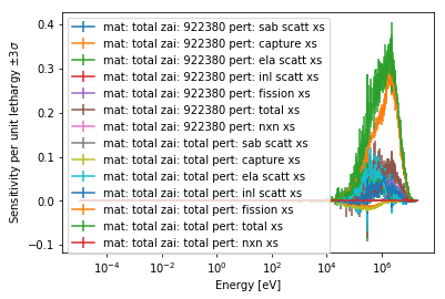
>>> sens.plot('keff');
The following arguments can be used to filter the data present:
key |
Action |
|---|---|
|
Isotopes(s) of interest |
|
Perturbation(s) of interest |
|
Material(s) of interest |
The sigma argument can be used to adjust the confidence interval
applied to the plot. The labelFmt argument can be used to modify the
label used for each plot. The following replacements will be made:
1. {r} - name of the response being plotted
1. {m} - name of the material
1. {z} - isotope zai
1. {p} - specific perturbation
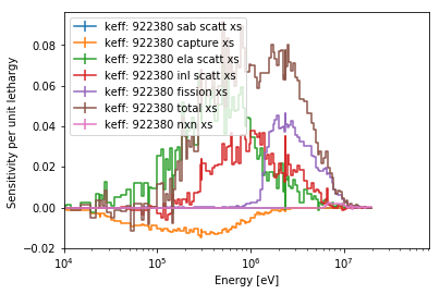
>>> ax = sens.plot('keff', 922380, mat='total', sigma=0,
...                labelFmt="{r}: {z} {p}")
>>> ax.set_xlim(1E4);  # set the lower limit to be closer to what we care about
The argument normalize is used to turn on/off normalization per unit
lethargy, while legend can be used to turn off the legend, or set
the legend outside the plot.
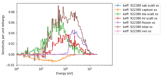
>>> ax = sens.plot('keff', 922380, mat='total', sigma=0,
...                labelFmt="{r}: {z} {p}", legend='right')
>>> ax.set_xlim(1E4);  # set the lower limit to be closer to what we care about
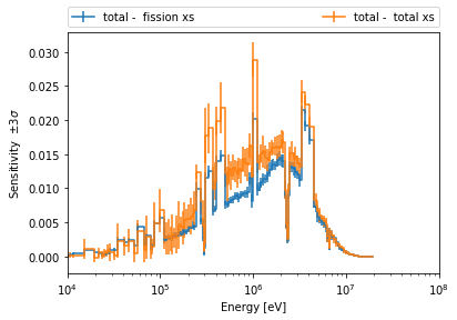
>>> sens.plot('keff', zai='total', pert=['total xs', 'fission xs'], labelFmt="{z} -  {p}",
...           legend='above', ncol=2, normalize=False)
>>> pyplot.xlim(1E4, 1E8);
Conclusion
The SensitivityReader can quickly read sensitivity files, and stores
all data present in the file. A versatile plot() method can be used to
quickly visualize sensitivities.
- gpt
Aufiero, M. et al. “A collision history-based approach to sensitivity/perturbation calculations in the continuous energy Monte Carlo code SERPENT”, Ann. Nucl. Energy, 152 (2015) 245-258.