Depletion Matrix Reader
Note
Data files, like the one used in this example, are not included with the
python distribution. They can be downloaded from the GitHub repository,
and accessed after setting the SERPENT_TOOLS_DATA environment
variable
>>> import os
>>> mtxFile = os.path.join(
...     os.environ["SERPENT_TOOLS_DATA"],
...     "depmtx_ref.m")
The serpentTools package supports reading depletion matrix files, generated when
set depmtx 1 is added to the input file. As of SERPENT 2.1.30, these files contain
The length of time for a depletion interval
Vector of initial concentrations for all isotopes present in the depletion problem
ZAI vector
Depletion matrix governing destruction and transmutation of isotopes
Vector of final concentrations following one depletion event
Files such as this are present for each burnable material tracked by SERPENT and
at each time step in the problem.
This document will demonstrate the DepmtxReader, designed to store such data.
Note
The depletion matrices can be very large for most problems, ~1000 x 1000 elements.
For this reason, the DepmtxReader can store matrices in
Compressed Sparse Column
or full numpy arrays. The reader will use the sparse format
if scipy is installed unless explicitely told to use dense arrays.
Basic Operation
>>> import serpentTools
>>> reader = serpentTools.read(mtxFile)
>>> reader
<serpentTools.parsers.depmatrix.DepmtxReader at 0x7f0b1a9702b0>
We now have access to all the data present in the file directly on the reader.
>>> reader.n0
array([1.17344222e-07, 6.10756908e-12, 7.48053806e-13, 7.52406757e-16,
       1.66113020e-34, 1.67580185e-09, 1.19223790e-36, 1.89040622e-26,
       5.09195054e-16, 7.91142112e-34, 1.68989876e-22, 6.92676695e-12,
       7.52406345e-16, 8.52076751e-13, 4.52429540e-02, 1.71307881e-12,
       1.86228871e-51, 2.32287315e-50, 1.15352152e-55, 7.72524686e-50,
       5.74084741e-44, 1.55414063e-42, 3.10757266e-40, 9.12566461e-40,
       6.82216144e-39, 9.71825616e-56, 1.59237444e-51, 1.14764875e-46,
       1.15203415e-43, 5.66072799e-41, 4.49411601e-34, 8.99210202e-31,
       8.65694179e-29, 5.96910982e-28, 1.06642058e-26, 9.10883647e-27,
       7.56006632e-36, 6.08157358e-33, 7.93562601e-40, 1.67857401e-29,
       2.76995718e-26, 2.42939173e-30, 6.93658246e-27, 3.21960435e-20,
       4.14863808e-17, 6.02145579e-16, 3.68254657e-15, 2.25927183e-15,
       2.85992932e-15, 5.34540710e-28, 2.34532631e-25, 1.36140065e-17,
       4.17935379e-16, 4.61527247e-15, 2.15346589e-15, 2.90307762e-15,
       4.90358169e-16, 3.62499544e-13, 4.61691784e-05, 2.96919439e-04,
       4.13730091e-04, 3.14746134e-04, 4.98296713e-04, 4.37637914e-04,
       3.84679634e-17, 6.87038906e-14, 4.29307714e-06, 5.62156587e-04,
       2.98288610e-08, 1.45634092e-09, 2.05487374e-02, 2.10836706e-07,
       9.84180195e-12, 8.05226656e-16], dtype=float128)
This specific input file did not include fission yield libraries and thus only tracks 74 isotopes, rather than 1000+, through depletion. This was intentionally done to reduce the size of files tracked in this project.
Number densities and entries in the depletion matrix are stored using the
numpy.longfloat data type to preserve the precision present in the output files.
>>> reader.zai
array([    -1,  10010,  10020,  10030,  20030,  20040,  30060,  30070,
        40090,  50100,  50110,  60120,  70140,  70150,  80160,  80170,
        561380, 561400, 581380, 581390, 581400, 581410, 581420, 581430,
        581440, 591410, 591420, 591430, 601420, 601430, 601440, 601450,
        601460, 601470, 601480, 601500, 611470, 611480, 611481, 611490,
        611510, 621470, 621480, 621490, 621500, 621510, 621520, 621530,
        621540, 631510, 631520, 631530, 631540, 631550, 631560, 631570,
        641520, 641530, 641540, 641550, 641560, 641570, 641580, 641600,
        922320, 922330, 922340, 922350, 922360, 922370, 922380, 922390,
        922400, 922410])
One can easily check if the depletion matrix is stored in a sparse or dense structure using the
sparse attribute:
>>> reader.sparse
True
>>> reader.depmtx
<74x74 sparse matrix of type ',class 'numpy.float128'>'
   with 633 stored elements in Compressed Sparse Column format>
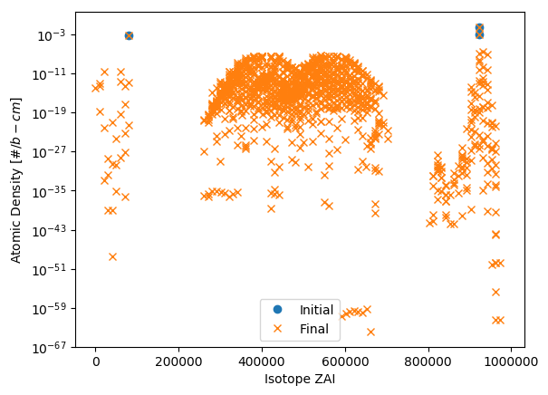
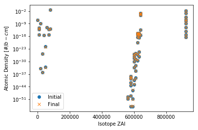
A simple plot method can be used to plot initial concentrations, final concentrations, or both:
>>> reader.plotDensity()
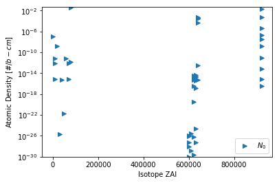
Some options can be passed to alter the formatting of the plot:
>>> reader.plotDensity(
      what='n0',  # plot only initial concentration
      markers='>',  # marker for scatter plot
      labels='$N_0$'  # label for each plotted entry
      ylim=1E-30,  # set the lower y-axis limit
   )
We can see that there is not a lot of change in the isotopic concentration in this depletion step. Furthermore, the classical fission yield distributions are not present due to the lack of fission yield data. Using a more complete, and typical data set, one can view the distribution of fission products more clearly, demonstrated in the below plot.