Cross Section Reader/Plotter

Note

Data files, like the one used in this example, are not included with the python distribution. They can be downloaded from the GitHub repository, and accessed after setting the SERPENT_TOOLS_DATA environment variable

>>> import os
>>> xfile = os.path.join(
...     os.environ["SERPENT_TOOLS_DATA"],
...     "plut_xs0.m")

Basic Operation

Firstly, to get started plotting some cross sections from Serpent, you generate a yourInputFileName_xs.m file using set xsplot as documented on the Serpent wiki. serpentTools can then read the output, figuring out its file type automatically as with other readers. Let’s plot some data used in the serpentTools regression suite.

>>> import serpentTools
>>> xsreader = serpentTools.read(xfile)

This file contains some cross sections from a Serpent case containing a chunk of plutonium metal reflected by beryllium. Let’s see what cross sections are available from the file:

>>> xsreader.xsections.keys()
dict_keys(['i4009_03c', 'i7014_03c', 'i8016_03c', 'i94239_03c', 'mbe',
'mfissile'])

Notice that the important part of the reader is the xsections attribute, which contains a dictionary of named XSData objects. Entries starting with “i” are isotopes, while “m” preceded names are materials. Notably, materials not appearing in the neutronics calculation, e.g., external tanks in Serpent continuous reprocessing calculations, are not printed in the yourInputFileName_xs.m file.

These XSData instances can be obtained by indexing into the xsections dictionary or the reader

>>> xsreader.xsections["i4009_03c"] is xsreader["i4009_03c"]
True

The final bit of useful information stored on the reader are the energy groups and majorant cross sections. The energy groups are shared across all XSData objects stored on the reader

>>> xsreader.energies
array([1.00000e-08, 1.03891e-07, 1.07934e-06, 1.12135e-05, 1.16498e-04,
       1.21032e-03, 1.25742e-02, 1.30635e-01, 1.35719e+00, 1.41000e+01])
>>> xsreader.majorant
array([78.4253  , 36.1666  ,  2.54417 , 13.0654  ,  4.27811 ,  0.822536,
       0.781066,  0.598564,  0.34175 ,  0.293887])

Data Access

Most of the useful information is stored on the XSData instances. These are primarily cross sections provided by Serpent and some descriptive data. The MT and MTdescrip attributes describe the ordering of the reactions and their descriptions

>>> o16 = xsreader["i8016_03c"]
# Make a quick dictionary to show descriptions
>>> dict(zip(o16.MT, o16.MTdescrip))
{1: 'Total',
 101: 'Sum of absorption',
 2: 'elastic scattering',
 ...
 105: '(n,t)',
 23: '(n,n3alpha)',
 16: '(n,2n)'}

Cross section data are stored in the xsdata array, which has shape (N_E, N_MT)

>>> o16.xsdata.shape == (len(o16.energies), len(o16.MT))
True

The data can be obtained in a few different ways. First, you can index into the array directly

>>> o16.xsdata[:, 0]
array([4.16597, 3.88237, 3.85502, 3.8523 , 3.8518 , 3.84938, 3.82434,
       3.58676, 3.19656, 1.593  ])

This does require you to know the position of your reaction. Alternatively, you can index into the XSData object using the reaction MT as a key

>>> o16[1]
array([4.16597, 3.88237, 3.85502, 3.8523 , 3.8518 , 3.84938, 3.82434,
       3.58676, 3.19656, 1.593  ])

The tabulate method can be used to create a pandas.DataFrame` for nice tabular representation.

>>> xsreader.xsections['mfissile'].tabulate()

	Energy (MeV)	MT -1 cm$^{-1}$	MT -3 cm$^{-1}$	MT -2 cm$^{-1}$	MT -6 cm$^{-1}$	MT -7 cm$^{-1}$	MT -16 cm$^{-1}$
0	1.000000e-08	78.425300	0.404950	19.669800	58.350500	167.674000	0.000000
1	1.038910e-07	36.166600	0.369643	12.045000	23.752000	68.055800	0.000000
2	1.079340e-06	2.544170	0.506089	0.410559	1.627520	4.672940	0.000000
3	1.121350e-05	13.065400	0.715384	2.015980	10.334000	29.525000	0.000000
4	1.164980e-04	4.278110	0.721668	0.434122	3.122320	9.000070	0.000000
5	1.210320e-03	0.822536	0.537059	0.003514	0.281963	0.814254	0.000000
6	1.257420e-02	0.781066	0.623379	0.047729	0.093854	0.271066	0.000000
7	1.306350e-01	0.583509	0.458020	0.010805	0.075165	0.217468	0.000000
8	1.357190e+00	0.341750	0.163555	0.000772	0.095130	0.291685	0.000000
9	1.410000e+01	0.293887	0.136424	0.000114	0.120609	0.596505	0.012848

Lastly, the descriptions for each reaction can be found in MTdescrip or using describe

>>> o16.MTdescrip[0]
'Total'
>>> o16.describe(1)
'Total'

Plotting

Plotting reactions is provided through the plot() method. With no MTs provided, all reactions are plotted and labeled

>>> be9 = xsreader['i4009_03c']
>>> be9.plot(legend='right');

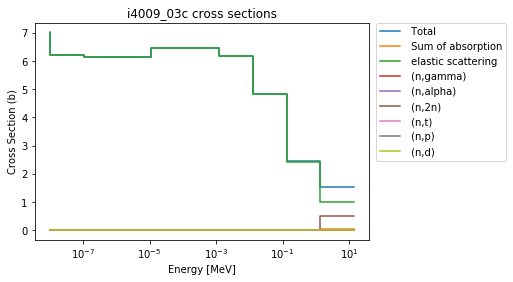
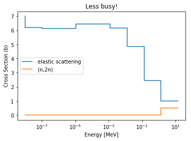
This is nice to have an automatically generated legend, but gets somewhat busy quickly. So, it’s easy to check which MT numbers are available, and plot only a few:

>>> be9.showMT()
MT numbers available for i4009_03c:
-----------------------------------
1     Total
101   Sum of absorption
2     elastic scattering
102   (n,gamma)
107   (n,alpha)
16    (n,2n)
105   (n,t)
103   (n,p)
104   (n,d)
>>> be9.plot(mts=[2, 16], title='Less busy!');

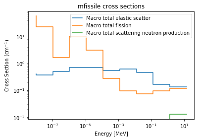
Of course, the same process can be applied to materials, but Serpent has some special unique negative MT numbers. The code will give you their meaning without requiring your reference back to the wiki.

>>> xsreader['mfissile'].showMT()
MT numbers available for mfissile:
----------------------------------
-1   Macro total
-3   Macro total elastic scatter
-2   Macro total capture
-6   Macro total fission
-7   Macro total fission neutron production
-16  Macro total scattering neutron production

>>> xsreader['mfissile'].plot(mts=[-3, -6, -16], loglog=True)

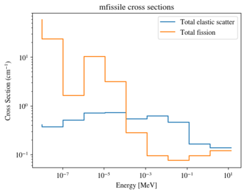
Labels can be configured through the labels argument

>>> xsreader['mfissile'].plot(
...     mts=[-3, -6], loglog=True,
...     labels=["Total elastic scatter", "Total fission"])

Conclusions

serpentTools can plot your Serpent XS data in a friendly way. We’re always looking to improve the feel of the code though, so let us know if there are changes you would like.

Keep in mind that setting an energy grid with closer to 10000 points makes far prettier XS plots however. There were none in this example to not clog up the repository.